Excelのアドイン機能を活用することで、普段よく行う操作をワンクリックでできるようになります。
今日は、テーブルの自動作成アドインを作っていきたいと思います。
このエクセルファイルの作り方
①マクロを使えるようにする(既に設定済の方は②に進んでください)
「マクロを使えるようにする」を参照
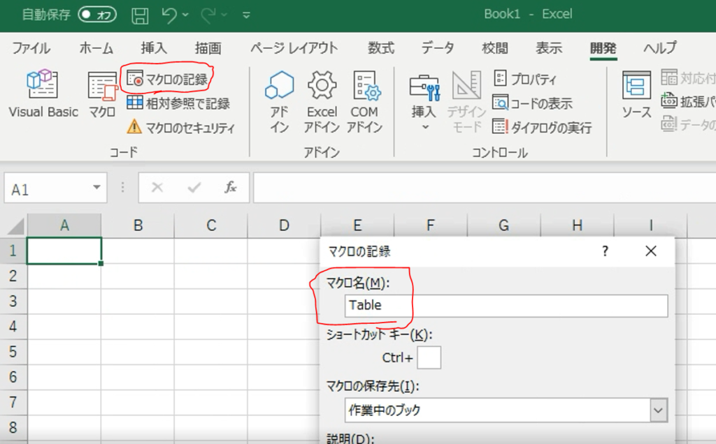
②「マクロの記録」ボタンを押します。(マクロ名は何でもいいですが、今回は「Table」とします)
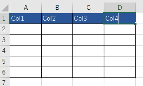
③テーブルを作成します
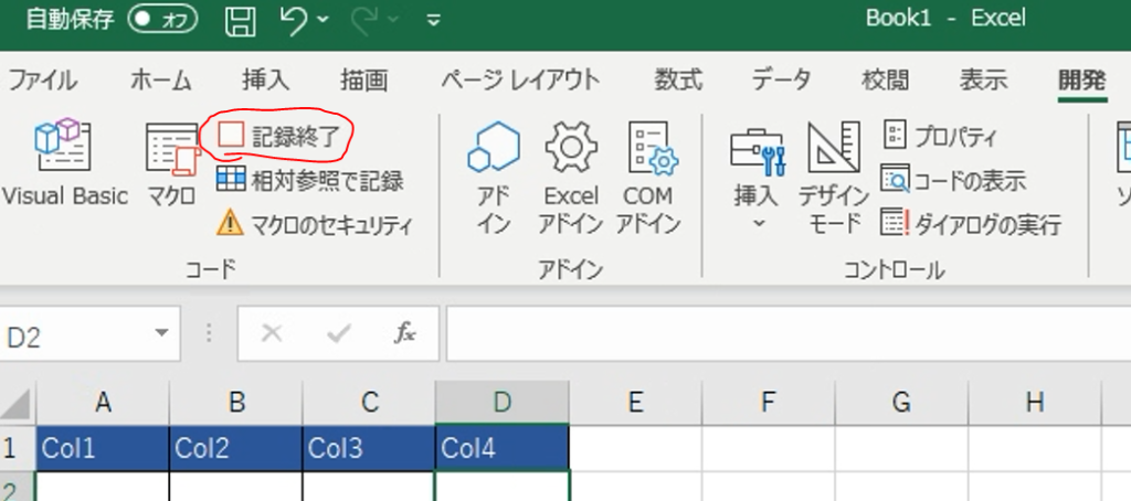
④「記録終了」を押します。
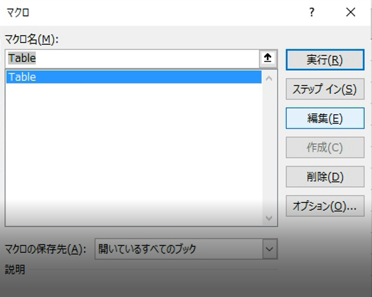
⑤「Alt + F8」を押して、「編集」を押します。(ソースコードが表示されます)
⑥ソースコードを微調整していきます。以下のソースをペーストします。
Sub Table()
    '特定のCellではなく選択範囲に罫線を描画する(Selectionというのが選択範囲)
    Selection.Borders(xlDiagonalDown).LineStyle = xlNone
    Selection.Borders(xlDiagonalUp).LineStyle = xlNone
    With Selection.Borders(xlEdgeLeft)
        .LineStyle = xlContinuous
        .ColorIndex = 0
        .TintAndShade = 0
        .Weight = xlThin
    End With
    With Selection.Borders(xlEdgeTop)
        .LineStyle = xlContinuous
        .ColorIndex = 0
        .TintAndShade = 0
        .Weight = xlThin
    End With
    With Selection.Borders(xlEdgeBottom)
        .LineStyle = xlContinuous
        .ColorIndex = 0
        .TintAndShade = 0
        .Weight = xlThin
    End With
    With Selection.Borders(xlEdgeRight)
        .LineStyle = xlContinuous
        .ColorIndex = 0
        .TintAndShade = 0
        .Weight = xlThin
    End With
    With Selection.Borders(xlInsideVertical)
        .LineStyle = xlContinuous
        .ColorIndex = 0
        .TintAndShade = 0
        .Weight = xlThin
    End With
    With Selection.Borders(xlInsideHorizontal)
        .LineStyle = xlContinuous
        .ColorIndex = 0
        .TintAndShade = 0
        .Weight = xlThin
    End With
    'タイトルを塗りつぶし(選択範囲の先頭行のみ)
    Range(Selection(1), Selection(1).Offset(0, Selection.Columns.Count - 1)).Select
    With Selection.Interior
        .Pattern = xlSolid
        .PatternColorIndex = xlAutomatic
        .ThemeColor = xlThemeColorAccent1
        .TintAndShade = -0.249977111117893
        .PatternTintAndShade = 0
    End With
    With Selection.Font
        .ThemeColor = xlThemeColorDark1
        .TintAndShade = 0
    End With
    'タイトルを描画(選択範囲の先頭行のみ)※これはなくてもいいです
    For col = Selection(1).Column To Selection(1).Offset(0, Selection.Columns.Count - 1).Column
        Cells(Selection(1).Row, col) = "Col" & col - Selection(1).Column + 1
    Next col
End Sub
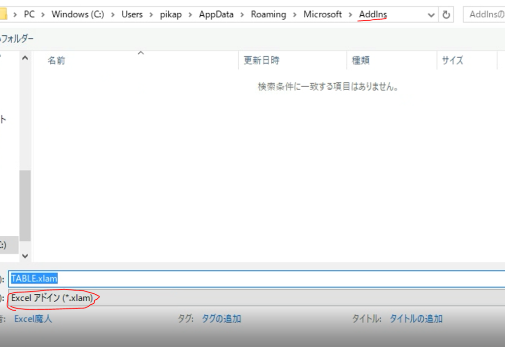
⑦ファイルの種類で「Excelアドイン(*.xlam)」を選択して保存します。
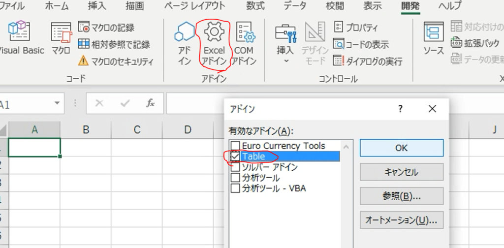
⑧「Excelアドイン」ボタンから、作成したアドイン(Table)を有効にします。
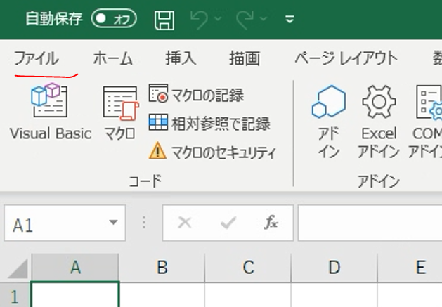
⑨「ファイル」を押します。
⑩「オプション」を押します。

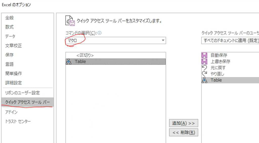
⑪「クイックアクセスツールバー」に今回作成した「Table」を追加します。
⑫「クイックアクセスツールバー」のボタンから、テーブルを自動作成できるようになります。
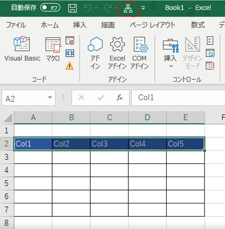
TABLE(AddIn)
1 file(s) 17.12 KB