最近ほとんど会社に行くことなく自宅でテレワークをしています。
今日はリモート会議で役立つ機能の紹介です。
↓のように、通常の設定だと赤枠の部分が人に見せる時には邪魔な事が多いです。
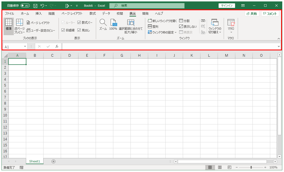
「Alt → V → U」と順番にキーボードを押すと、↓のように全画面表示にすることができます。
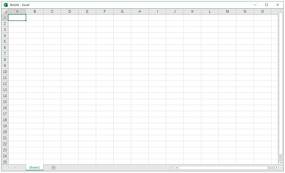
元に戻したい時は「Esc」キーを押します。
Excelで情報共有しており、Excelに追記した内容をメールで共有するケースがあるかと思います。
面倒なメール作成を自動でできるようにしてみました。
件名やメール本文は微調整してご利用ください。
①マクロを使えるようにする
「マクロを使えるようにする」を参照
②ボタンを配置する
※ ボタンの配置方法は「表を複数の条件で絞り込む②」を参照
③ボタン配置時の以下の画面で「マクロ名」を「CreateEmail」として「新規作成」を押す
④ 「Microsoft Visual Basic for Applications」にて以下のコードを記載
Sub CreateEmail()
Dim oApp As Object
Dim objMAIL As Object
Dim messageList(1) As String
Dim n As Long
Dim fullName As String
Dim firstName As String
On Error Resume Next
Set oApp = GetObject(, "Outlook.Application")
On Error GoTo 0
If oApp Is Nothing Then
Set oApp = CreateObject("Outlook.Application")
oApp.GetNamespace("MAPI").GetDefaultFolder(6).display
End If
fullName = Application.UserName
firstName = Mid(fullName, 1, InStr(fullName, " ") - 1)
Set objMAIL = oApp.CreateItem(0)
'メールに載せるメッセージ本文'
messageList(0) = "お疲れ様です。" & firstName & "です。" & vbCrLf & vbCrLf & _
"共有ファイルNo." & Cells(3, 3).Value & "に追記を行いました。" & vbCrLf & _
"タイミングを見てご確認ください。" & vbCrLf & vbCrLf & _
"<\ShareServer\メールを自動作成する.xlsm>" &amp; vbCrLf
messageList(1) = vbCrLf &amp; " 以上、宜しくお願い致します。"
Dim adress As String
Dim i As Long
For i = 1 To 50
adress = adress + ThisWorkbook.Worksheets("宛先").Cells(i + 1, 2).Value
adress = adress + " ;"
Next i
objMAIL.To = adress
'件名'
objMAIL.Subject = "共有ファイルNo." &amp; Cells(3, 3).Value &amp; "を追加しました"
objMAIL.BodyFormat = 2 'HTML形式
objMAIL.Body = messageList(0) &amp; messageList(1)
objMAIL.display
n = Len(messageList(0))
ActiveSheet.Range(Cells(Cells(3, 3) + 5, 2), Cells(Cells(3, 3) + 5, 5)).Copy
oApp.ActiveInspector.WordEditor.Range(n, n).Paste
Application.CutCopyMode = False
Set objMAIL = Nothing
Set oApp = Nothing
End Sub
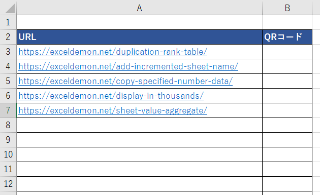
「Google Charts API」を利用して、URL等を一括でQRコードにするプログラムを作成します。
商品パッケージやパンフレットなどへの添付にご活用ください。
①マクロを使えるようにする
「マクロを使えるようにする」を参照
②URL、QRコードの表を作成
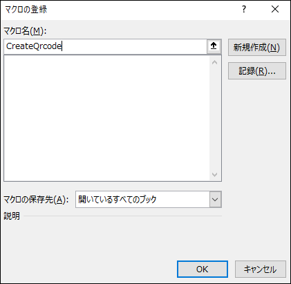
③ボタン配置時の以下の画面で「マクロ名」を「CreateQrcode」として「新規作成」を押す
④Microsoft Visual Basic for Applications」にて以下のコードを記載
Sub CreateQrcode()
'開始行
Dim firstRow As Long: firstRow = 3
'最終行の取得
Dim lastRow As Long: lastRow = Cells(Rows.Count, 1).End(xlUp).Row
'firstRow~lastRowまで繰り返し(途中エラーが出た場合も止めずに最後まで処理)
On Error Resume Next
For i = firstRow To lastRow
'QRコード表示セルの高さなどを調整
With Cells(i, "B")
.RowHeight = 65
.VerticalAlignment = xlTop '上詰め
End With
'GoogleAPIでQRコードを作成
Set qr = ActiveSheet.Pictures _
.Insert("http://chart.apis.google.com/chart?cht=qr&amp;amp;amp;amp;chs=80x80&amp;amp;amp;amp;chl=" _
+ Cells(i, "A").Value)
'QRコードの表示位置を指定
With qr
.Top = Cells(i, "B").Top + 2
.Left = Cells(i, "B").Left + 2
End With
Next i
On Error GoTo 0
End Sub
売上データなど、Excelで作った表を送る場合に、メールやチャットにてテキスト形式で送りたいことがあると思います。
そんなExcel表からテキストへ変換するためのプログラムを作成してみました。
私はシステムエンジニアなので、プログラムのコメントでテキスト形式の表を書いたりします。
今回は、範囲選択した中のデータをテキスト形式の表にし、クリップボードにコピーします。(メモ帳等に張り付けてご利用ください)
なお、セルの書式設定が通貨(#,##0)の場合のみ三桁カンマを付与し、値が数値の場合は右寄せ、それ以外は左寄せで表を作成します。
①マクロを使えるようにする
「マクロを使えるようにする」を参照
②ボタンを配置する
※ ボタンの配置方法は「表を複数の条件で絞り込む②」を参照
③ボタン配置時の以下の画面で「マクロ名」を「ConvertTable 」として「新規作成」を押す
④ 「Microsoft Visual Basic for Applications」にて以下のコードを記載
Sub ConvertTable()
Dim result As String
Dim startRow, startCol, endRow, endCol As Integer
Dim selectArea As Range
Set selectArea = Selection
startRow = selectArea.Cells(1).Row
startCol = selectArea.Cells(1).Column
endRow = selectArea.Cells(selectArea.Count).Row
endCol = selectArea.Cells(selectArea.Count).Column
Dim widthDic As Object
Set widthDic = CreateObject("Scripting.Dictionary")
Dim maxWidth As Integer: maxWidth = 0
Dim cellVal As String
Dim margin As Integer
' 各列毎の最大幅を配列で保持
For j = startCol To endCol Step 1
For i = startRow To endRow Step 1
cellVal = Cells(i, j).Value
If IsNumeric(cellVal) And Cells(i, j).NumberFormatLocal = "#,##0" Then
cellVal = Format(cellVal, "#,#")
End If
If maxWidth < LenB(StrConv(cellVal, vbFromUnicode)) Then
maxWidth = LenB(StrConv(cellVal, vbFromUnicode))
End If
Next
widthDic.Add j, maxWidth
maxWidth = 0
Next
' 表文字列の作成
For i = startRow To endRow Step 1
' 線だけの行を書き込み
For j = startCol To endCol Step 1
If i = startRow Then
If j = startCol Then
result = result & "┌"
Else
result = result & "┬"
End If
Else
If j = startCol Then
result = result & "├"
Else
result = result & "┼"
End If
End If
result = result & String(Application.WorksheetFunction.RoundUp(widthDic.Item(j) / 2, 0), "─")
If i = startRow And j = endCol Then
result = result & "┐"
ElseIf i <> startRow And j = endCol Then
result = result & "┤"
End If
Next
result = result & vbCrLf
' 値の行を書き込み
For j = startCol To endCol Step 1
result = result & "│"
cellVal = Cells(i, j).Value
If IsNumeric(cellVal) And Cells(i, j).NumberFormatLocal = "#,##0" Then
cellVal = Format(cellVal, "#,#")
End If
margin = widthDic.Item(j) - LenB(StrConv(cellVal, vbFromUnicode))
margin = margin + widthDic.Item(j) Mod 2
If IsNumeric(cellVal) Then
result = result & Space(margin)
result = result & cellVal
Else
result = result & cellVal
result = result & Space(margin)
End If
If j = endCol Then
result = result & "│"
End If
Next
result = result & vbCrLf
Next
' 最下部の線を書き込み
For j = startCol To endCol Step 1
If j = startCol Then
result = result & "└"
Else
result = result & "┴"
End If
result = result & String(Application.WorksheetFunction.RoundUp(widthDic.Item(j) / 2, 0), "─")
If j = endCol Then
result = result & "┘"
End If
Next
'表文字列をクリップボードに格納する
With New MSForms.DataObject
.SetText result
.PutInClipboard
End With
End Sub
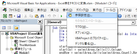
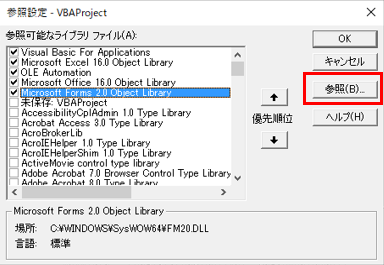
⑤ 「C:\Windows\System32\FM20.DLL」を参照する
※クリップボードに値を格納するためのアセンブリ
※ない場合は 「C:\Windows\SysWOW64\FM20.DLL」
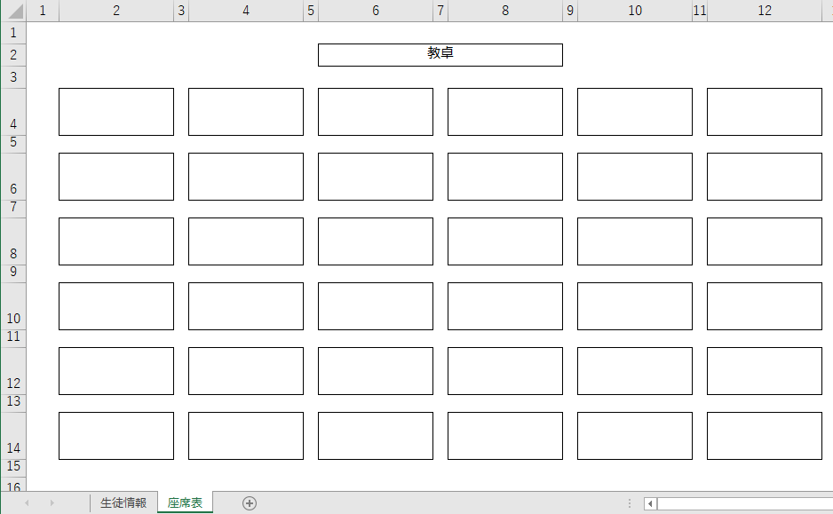
背の小さい順や成績の悪い順で、座席を割り振りたいケースがあると思います。
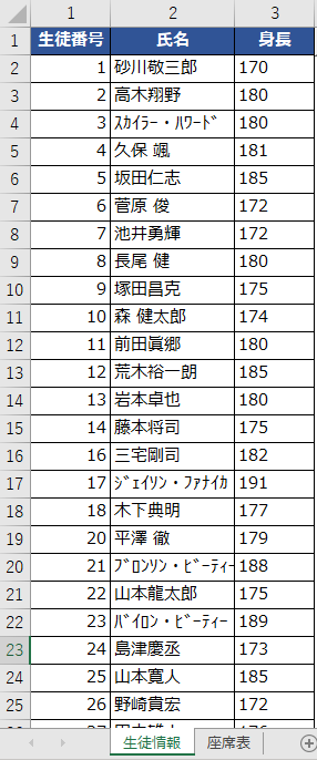
今回は生徒の名簿一覧から背の順で座席を割り振る方法を紹介させて頂きます。
①マクロを使えるようにする
「マクロを使えるようにする」を参照
②生徒情報の表を作成
③座席表を作成
④席決め配置ボタンを配置する
※ ボタンの配置方法は「表を複数の条件で絞り込む②」を参照
⑤ボタン配置時の以下の画面で「マクロ名」を「 StartSeatSelection 」として「新規作成」を押す
⑥「Microsoft Visual Basic for Applications」にて以下のコードを記載
Sub StartSeatSelection()
Dim noCol As Integer: noCol = 1 '★
Dim nameCol As Integer: nameCol = 2 '★
Dim heightCol As Integer: heightCol = 3 '★
Dim startRow As Integer: startRow = 2 '★
Dim lastRow As Integer: lastRow = ActiveSheet.UsedRange.Row + ActiveSheet.UsedRange.Rows.Count - 1
Dim studentList As Dictionary
Set studentList = New Dictionary
Dim tempStudentList As Dictionary
Set tempStudentList = New Dictionary
'「生徒情報」シートの内容を1行ずつ読み込み、studentListに身長順で格納します。
For i = startRow To lastRow Step 1
Set tempStudentList = studentList
Set studentList = New Dictionary
Dim no As String
no = Cells(i, noCol).Value
Dim name As String
name = Cells(i, nameCol).Value
Dim height As String
height = Cells(i, heightCol).Value
If IsEmpty(no) Then
MsgBox "生徒番号が空欄です。"
End If
If Not IsNumeric(no) Then
MsgBox no &amp; ":生徒番号には数値を指定してください。"
End If
If IsEmpty(name) Then
MsgBox "氏名が空欄です。"
End If
If IsEmpty(height) Then
MsgBox "身長が空欄です。"
End If
If Not IsNumeric(height) Then
MsgBox height &amp; ":身長には数値を指定してください。"
End If
If tempStudentList.Count &gt; 0 Then
For Each tempStudent In tempStudentList.Items
If (tempStudent(2) &gt; height Or (tempStudent(2) = height And tempStudent(0) &gt; no)) And Not studentList.Exists(no) Then
studentList.Add no, Array(no, name, height)
End If
studentList.Add tempStudent(0), Array(tempStudent(0), tempStudent(1), tempStudent(2))
Next tempStudent
End If
If Not studentList.Exists(no) Then
studentList.Add no, Array(no, name, height)
End If
Next
'studentListを基に、座席に名前をあてはめます。
Dim startSheetRow As Integer: startSheetRow = 4 '★
Dim lastSheetRow As Integer: lastSheetRow = 14 '★
Dim startSheetCol As Integer: startSheetCol = 2 '★
Dim lastSheetCol As Integer: lastSheetCol = 12 '★
Dim targetRow As Integer
Dim targetCol As Integer
Dim studentListCnt As Integer: studentListCnt = 0 '★
For targetRow = startSheetRow To lastSheetRow Step 2
For targetCol = startSheetCol To lastSheetCol Step 2
Worksheets("座席表").Cells(targetRow, targetCol).Value = studentList.Items(studentListCnt)(1)
studentListCnt = studentListCnt + 1
Next targetCol
Next targetRow
End Sub